Introduction
The purpose of this project is to find an efficient implementation of PCG32 2 PRNG algorithm on CUDA-enabled GPUs. Main focus lies on providing a CUDA kernel, which fills an array in device memory with generated numbers in the same order as a classical CPU implementation would.
This paper will not analyse the statistical or cryptographic properties of PCG family generators. Nor will it compare the performance to other PRNG algorithms. It’s focus lies on finding the fastest implementation of PCG32 algorithm.
PCG32
The minimal PCG32 standard specifies that internal state of the generator consists of two 64-bit integers denoted and respectively. These integers are the seed of the generated sequence. remains constant throughout the lifetime of generator and changes with each produced number. The standard also defines a constant .
Two functions that are used to generate a series of random numbers based on the internal state are:
-
The state-transition function: which offsets generator state by 1.
-
And the output function which takes and produces one pseudo-random 32-bit number.
Algorithm
General idea
We can generalise the state offset function to allow for any positive offset like so: Aside from this function also takes a second argument - .
Output function, while defined by PCG32 standard, is not important in context of efficient sequence generation since its complexity is constant and its result is a pseudo-random number, which is not used to calculate subsequent numbers.
This means that efficiently generating the random sequence, translates to generating the sequence of values of , which breaks down to calculating the subsequent powers: and sums: .
Brown’s algorithm
In order to calculate faster than naively (linear complexity) we can utilise Brown’s algorithm 1 which has the complexity of . It can be thought of as an extension to the well-known fast integer exponentiation algorithm.
sum = 0
power = 1
increment = 1
multiplier = M
while (n != 0)
    if (n % 2 == 1)
        power = power * multiplier
        sum = sum * multiplier + increment
    increment = increment * (multiplier + 1)
    multiplier = multiplier * multiplier
    n = n / 2
S = S * power + I * sum
One-number-per-thread approach
To generate random numbers a classic CPU implementation would perform only operations. This is because linear single-thread algorithm calculates each value of only once and immediately uses it to calculate .
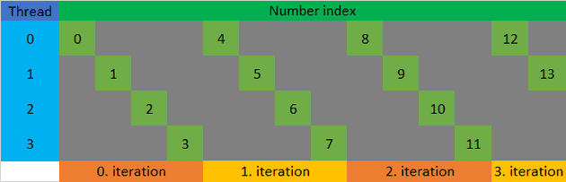
On the other hand, if we execute a CUDA kernel, where each thread calculates one random number using Brown’s algorithm, each thread would perform operations. That gives in total operations, which is not work-efficient, because most computations are repeated by different threads. For instance half of the threads would calculate and a quarter would calculate as intermediary values while calculating their target , where is the thread’s index. Profiling also shows that this approach’s performance is limited by computation throughput.
Multi-linear approach
Once and have been calculated for particular they can be reused. Which means generating a sequence requires only multiplications and additions aside from the initial calculations of and .
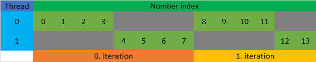
If in a CUDA kernel each thread generates out of random numbers (see figure 1), we can use Brown’s algorithm to calculate and just once. Such kernel would be composed of threads, each of which would calculate their own and then using and generate the sequence . In total all threads would perform operations. This means work-efficiency increases as number of threads decreases, but at a cost of parallelism.
Parallelism, i.e. maximum number of concurrent threads, is still limited on a GPU, despite being many orders of magnitudes bigger than on a CPU. If a multi-linear kernel is tuned to utilise all of its cores while not creating too many threads, we can achieve maximum performance.
Optimisations
Profiling shows that utilising vectorized memory access allows for better interleave of computations and memory stores, which in turn yields a small performance increase.
It is also worth noting that multi-linear approach is the most efficient when is a power of 2. This is because Brown’s algorithm is based on treating the exponent as a sum of powers of 2, which means that and are simply the values of and after the loop iteration. If is not a power of 2 then it is necessary to use Brown’s algorithm twice - once to calculate and once to calculate and , unless an optimal (potentially GPU-specific) is hard-coded and these two values are precomputed.
Additionally the and for each iteration of Brown’s algorithm can be precomputed and loaded to GPU’s constant memory. If we limit the number of iterations to 16 (thus limiting the number of threads to ) then storage of these constants takes only bytes.
Implementation
Fragments of source code included in this paper have been adapted for readability from benchmarked implementation of multi-linear approach 4. For benchmark results see section 2.6.
This implementation takes initial generator state ( and ) as an argument and does not return final generator state (). However it is simple to modify it to read from device memory and/or write to device memory for subsequent kernel to utilise. Alternatively a global offset to generated numbers’ indices can be easily added as a kernel parameter.
Assumptions
Code presented below makes use of pcg32_random_t type, which is used
by official PCG32 minimal C implementation 3, to
represent a generator instance containing its internal state and
referenced as .state and .inc.
These code listings also assume all proposed optimisations
(2.4.1) are present, i.e. memory access is
vectorized, number of threads is a power of 2 and there exist two
globally accessible constant arrays: uint64_t multipliers[] and
uint64_t increments[], which are populated with precomputed values for
consecutive iterations of Brown’s algorithm.
Output function
uint32_t pcg32_xsr(uint64_t state)
{
    uint32_t xsh = (uint32_t)(((state >> 18u) ^ state) >> 27u);
    uint32_t rot = state >> 59u;
    return (xsh >> rot) | (xsh << ((-rot) & 31));
}
Brown’s algorithm
void offset_state(pcg32_random_t &gen, int64_t index)
{
    uint64_t power = gen.state;
    uint64_t sum = 0;
    for (int it = 2; index != 0; it++, index >>= 1)
    {
        if (index & 1)
        {
            power = power * multiplier[it];
            sum = sum * multiplier[it] + increment[it];
        }
    }
    gen.state = power + gen.inc * sum;
}
Note the ”int it = 2” within loop initialisation. This makes each
thread calculate instead of as its starting state.
Multi-linear approach
void generate_numbers(uint32_t *results, pcg32_random_t gen, int64_t index,
                      const int64_t numbers, const int threads_log2)
{
    const int64_t step = 1LL << threads_log2;
    while (index * 4 + 3 < numbers)
    {
        uint4 result_vec;
        uint64_t s = gen.state;
        result_vec.x = pcg32_xsr(s);
        s = s * multiplier[0] + gen.inc;
        result_vec.y = pcg32_xsr(s);
        s = s * multiplier[0] + gen.inc;
        result_vec.z = pcg32_xsr(s);
        s = s * multiplier[0] + gen.inc;
        result_vec.w = pcg32_xsr(s);
        ((uint4*)results)[index] = result_vec;

        gen.state = gen.state * multiplier[threads_log2]
                    + gen.inc * increment[threads_log2];
        index += step;
    }
    for (int i = 0; index * 4 + i < numbers; i++)
    {
        results[index * 4 + i] = pcg32_xsr(gen.state);
        gen.state = gen.state * multiplier[0] + gen.inc;
    }
}
Kernel
void kernel(uint32_t *results, pcg32_random_t gen,
            const int64_t numbers, const int threads_log2)
{
    const int64_t index = threadIdx.x + blockIdx.x * (int64_t)blockDim.x;
    offset_state(gen, index);
    generate_numbers(results, gen, index, numbers, threads_log2);
}
Benchmarks
Presented here are the results of benchmarks of multi-linear approach with all proposed optimisations implemented. For technical specification of benchmark setup see section 2.6.1.
![Average time [ps] per number in a multi-linear kernel generating
2^{30} numbers. Time values are placed on a logarithmic scale (base 2)
grouped by threads in a
kernel.](/static/07d36d0c7b90f8b8845ffe14e9b9e872/f058b/benchmark-by-threads.png)
Figure 3 shows, that time per number generated is the smallest when total number of threads in a kernel is between and . Below this range the GPU cannot be fully utilised, while above it the computational cost of repeated work becomes significant.
In order to measure GPU’s memory throughput a simple kernel was benchmarked, where each thread stores a single 4x4-byte vector to device memory. Total memory usage is equal to amount of memory, which numbers generated by corresponding multi-linear kernel occupy.
![Average execution time [ns] of a multi-linear kernel with 2^{14}
threads in a kernel. "Throughput" kernel for reference. Time values
are placed on a logarithmic scale (base 2) grouped by numbers
generated.](/static/c9f213d5dd4f5aa3edd397ef619ed83a/f058b/benchmark-by-numbers.png)
The results of benchmarks show that multi-linear kernel’s execution time is comparable to that of the “throughput” kernel. This proves that multi-linear algorithm is close to achieving maximum GPU throughput.
Technical specifications of machines, on which benchmarks were performed
| GPU | VRAM | CPU | RAM |
|---|---|---|---|
| 1x Tesla K20m | 1x 5 GiB | 2x Intel Xeon E5649 | 15 GiB |
| 4x Tesla P100 | 4x 16 GiB | 2x Intel Xeon E5-2695 v4 | 512 GiB |
| 8x NVIDIA A100-SMX4 | 8x 40 GiB | 2x AMD EPYC 7742 64-Core | 1 TiB |
Table: Technical specifications of benchmark machines
While the machines may be equipped with more than one CPU or GPU, benchmark utilised only one of each.
Rejected ideas
Alternative to Brown’s algorithm
An alternative algorithm with logarithmic complexity was developed to calculate the offset state , but, despite being more complex, it was less efficient. The algorithm was based on following observations:
-
Sum of geometric series:
-
, so here:
-
From Chinese remainder theorem 5:
where and (Bézout’s identity) -
, so
To calculate , first lower 66 bits of were computed and then, using reasoning explained above, was calculated. This algorithm required extended precision integer arithmetic, including division, which was implemented using Barret’s algorithm. The benchmarked version featured multiple optimisations including PTX routines for arithmetic, but was unable to match the performance of Brown’s algorithm.
Opportunistic reuse of calculated offset states
In order to reduce the overlap (i.e. identical computations) between calculations of different threads an idea was explored for threads to publish calculated offset states to global memory. When a new block began execution it would use the latest block’s published states as basis for its own offset state calculations.
This solution did provide performance gain over one-number-per-thread approach, but required reading and storing 8-byte values to global memory, which was significantly slower than multi-linear approach which only performs 4-byte stores. Another downside is the need for second stage kernel which would perform the final calculation of random numbers from published sequence of states, i.e. apply PCG32 output function.
Summary
The goal of this project has been accomplished. Proposed implementation 4 provides a way to generate a sequence of PCG32 random numbers on a CUDA-enabled GPU in the same order as a CPU implementation. It achieves perfect coalescing and very high utilisation of memory bandwidth, which results in near-speed-of-light performance. Work-efficiency is also similar to the linear approach, with overhead depending only on the number of threads in the kernel.
Bibliography
-
- 1.Melissa E. O’Neill. PCG: A Family of Simple Fast Space-Efficient Statistically Good Algorithms for Random Number Generation. Tech. rep. HMC-CS-2014-0905. Claremont, CA: Harvey Mudd College, Sept. 2014. url: https://www.cs.hmc.edu/tr/hmc-cs-2014-0905.pdf
-
- 2.Forrest B. Brown. Random number generation with arbitrary strides. In: Transactions of the American Nuclear Society 71.ISSN 0003-018X (Dec. 1994), pp. 202–203. url: https://www.osti.gov/biblio/89100
-
- 4.Patryk Pochmara. CUDA PCG32. Github Repository. 2024. url: https://github.com/Patonymous/cuda-pcg32
-
- 3.Melissa E. O’Neill. PCG32 minimal C implementation. [Accessed 21-May-2024]. 2018. url:https://www.pcg-random.org/download.html#minimal-c-implementation
-
- 5.K. H. Rosen. Elementary Number Theory and Its Applications. 1993. url: https://books.google.pl/books?id=gfnuAAAAMAAJ